
In statistics, the uniform distribution, also known as the rectangular distribution, is a type of probability distribution where every possible outcome is equally likely. Imagine picking a number at random from a given range – that’s a uniform distribution in action. This distribution is characterized by its simplicity and is often used to model scenarios where all outcomes within a certain interval are considered equally probable.
While the concept of uniform distribution itself is straightforward, understanding its statistical measures, such as the standard deviation, is crucial for data analysis and interpretation. The standard deviation, in essence, measures the dispersion or spread of a dataset around its mean. For a uniform distribution, it tells us how much the values are spread out across the defined range.
Let’s delve into calculating and understanding the Standard Deviation Of A Uniform Distribution using a practical example.
Uniform Distribution: Repair Time Example
Consider a scenario from Ace Heating and Air Conditioning Service. They’ve observed that the time their repairmen take to fix a furnace is uniformly distributed between 1.5 and 4 hours. If we denote the time needed to fix a furnace as (x), we can represent this as (x sim U(1.5, 4)).
Let’s explore some common questions related to this uniform distribution:
1. Probability of Repair Time Exceeding Two Hours
What is the probability that a randomly selected furnace repair takes more than two hours?
To solve this, we first need to define the probability density function (PDF) for a uniform distribution. For a uniform distribution (U(a, b)), the PDF, (f(x)), is given by:
[ f(x) = frac{1}{b-a} ]
for (a leq x leq b), and (f(x) = 0) otherwise.
In our case, (a = 1.5) and (b = 4), so:
[ f(x) = frac{1}{4-1.5} = frac{1}{2.5} = 0.4 ]
Thus, (f(x) = 0.4) for (1.5 leq x leq 4).
The probability (P(x > 2)) is the area under the PDF curve from (x = 2) to (x = 4). For a uniform distribution, this area is simply the area of a rectangle:
[ P(x > 2) = text{base} times text{height} = (4 – 2) times 0.4 = 0.8 ]
Therefore, there is an 80% probability that a furnace repair will take more than two hours.
 Uniform Distribution between 1.5 and four with shaded area between two and four representing the probability that the repair time x is greater than two
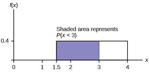
2. Probability of Repair Time Being Less Than Three Hours
What is the probability that a randomly selected furnace repair requires less than three hours?
Similarly, we need to find the probability (P(x < 3)). This is the area under the PDF curve from (x = 1.5) to (x = 3):
[ P(x < 3) = text{base} times text{height} = (3 – 1.5) times 0.4 = 0.6 ]
So, there is a 60% probability that a furnace repair will take less than three hours.
Uniform Distribution between 1.5 and four with shaded area between two and four representing the probability that the repair time x is greater than two
3. Finding the 30th Percentile of Repair Times
The 30th percentile represents the value below which 30% of the data falls. In terms of repair times, we want to find the time (k) such that (P(x (0.3 = (k – 1.5) times (0.4))
Solving for (k):
[ frac{0.3}{0.4} = k – 1.5 ]
[ 0.75 = k – 1.5 ]
[ k = 0.75 + 1.5 = 2.25 ]
The 30th percentile of furnace repair times is 2.25 hours. This means 30% of repair times are 2.25 hours or less.
Uniform Distribution between 1.5 and four with shaded area between two and four representing the probability that the repair time x is greater than two
4. Determining the Longest 25% of Repair Times
We want to find the minimum time for the longest 25% of repair times. This is equivalent to finding the 75th percentile, or the value (k) such that (P(x > k) = 0.25).
[ P(x > k) = (4 – k) times 0.4 = 0.25 ]
Solving for (k):
[ frac{0.25}{0.4} = 4 – k ]
[ 0.625 = 4 – k ]
[ k = 4 – 0.625 = 3.375 ]
The longest 25% of furnace repairs take at least 3.375 hours. This also means that 3.375 hours represents the 75th percentile of furnace repair times.
5. Mean and Standard Deviation of Uniform Distribution
Finally, let’s calculate the mean ((mu)) and the standard deviation ((sigma)) for this uniform distribution. For a uniform distribution (U(a, b)), the formulas are:
Mean:
[ mu = frac{a+b}{2} ]
Standard Deviation:
[ sigma = sqrt{frac{(b-a)^{2}}{12}} ]
For our furnace repair time distribution (U(1.5, 4)):
Mean:
[ mu = frac{1.5 + 4}{2} = frac{5.5}{2} = 2.75 ]
The mean repair time is 2.75 hours.
Standard Deviation:
[ sigma = sqrt{frac{(4 – 1.5)^{2}}{12}} = sqrt{frac{(2.5)^{2}}{12}} = sqrt{frac{6.25}{12}} approx sqrt{0.5208} approx 0.7217 ]
The standard deviation of the furnace repair time is approximately 0.7217 hours. This value indicates the typical deviation of repair times from the average repair time of 2.75 hours. A smaller standard deviation would imply that repair times are more clustered around the mean, while a larger standard deviation suggests a wider spread.
Conclusion
Understanding the standard deviation of a uniform distribution is essential for grasping the variability within uniformly distributed data. In the context of our furnace repair example, the standard deviation of approximately 0.7217 hours provides a measure of how much the repair times vary around the average of 2.75 hours. This knowledge is valuable for service scheduling, customer expectation management, and resource allocation for Ace Heating and Air Conditioning Service. By using simple formulas, we can easily calculate and interpret key statistical measures for uniform distributions, making them a practical tool in various analytical scenarios.