In the realm of statistical genetics, accurately interpreting p-values is crucial for drawing meaningful conclusions from experimental data. A biologist encountered an intriguing problem while applying Fisher’s exact test in a simulated genetics scenario, observing a perplexing right-skewed distribution of p-values. This observation deviates from the theoretical expectation of a uniform distribution under the null hypothesis, prompting an investigation into the potential causes and interpretations, particularly concerning what might be termed “Fishers Uniform” distribution.
The initial setup involved generating two independent samples of binary data (0s and 1s) in R, each with 500 observations and equal probabilities for 0 and 1. Applying Fisher’s exact test to compare the proportions within these samples across 30,000 iterations yielded a p-value distribution that was surprisingly skewed to the right.
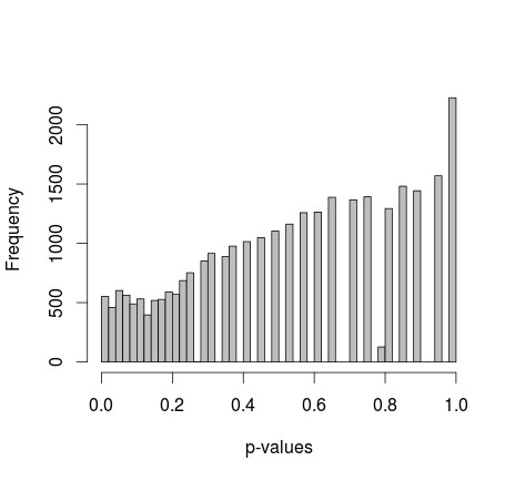 p-value distribution
The mean p-value was notably around 0.55, with the 5th percentile at 0.0577. This distribution, seemingly discontinuous on the right, raised questions about whether this behavior was statistically normal or indicative of an underlying issue in the experimental design or analysis. The core question revolved around understanding if this deviation from a uniform distribution, or “fishers uniform,” was expected, a result of small sample sizes, or a misinterpretation of p-values.
Seeking to refine the simulation and potentially achieve a more “fishers uniform” outcome, a modification was introduced to fix the marginal totals of 0s and 1s. This adjustment, aiming to constrain the sample space, led to a noticeable change in the p-value distribution.
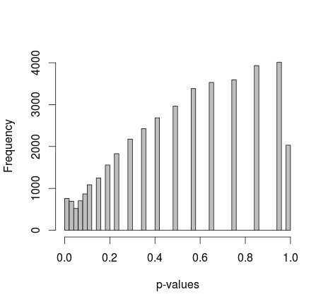 p-vals w fixed marginals
The R code implemented for this revised setup was:
samples=c(rep(1,500),rep(2,500))
alleles=c(rep(0,500),rep(1,500))
p=NULL
for(i in 1:30000){
  alleles=sample(alleles)
  p[i]=fisher.test(samples,alleles)$p.value
}
hist(p,breaks=50,col="grey",xlab="p-values",main="")
While this modification shifted the p-value distribution, it did not result in a perfectly uniform distribution, nor one that immediately conformed to a recognizable shape. This raised further questions about the nature of “fishers uniform” and the factors influencing p-value distributions in Fisher’s exact test.
However, a crucial insight emerged upon closer examination of the histograms: the apparent non-uniformity, particularly the “discontinuities,” could be an artifact of binning in the histogram visualization. To address this, QQ-plots were employed to provide a more accurate assessment of uniformity.
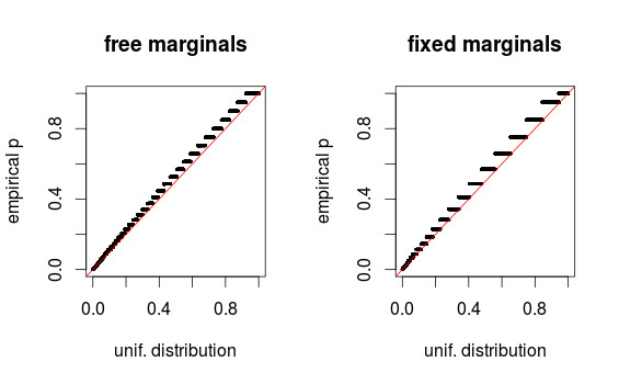 pval-qqplot
The QQ-plots for both the initial setup (free marginals) and the modified setup (fixed marginals) revealed that the p-value distributions were, in fact, reasonably uniform. This demonstrated that the perceived skew and non-uniformity from the histograms were largely due to visual distortion from binning. The QQ-plots effectively confirmed that the p-values, in both scenarios, aligned with the expectation of a “fishers uniform” distribution under the null hypothesis, highlighting the importance of choosing appropriate visualization methods for statistical distributions and the nuanced interpretation of “fishers uniform” in statistical testing.