In probability and statistics, the Uniform Random Variable stands as a fundamental concept, characterized by the property that all outcomes within its range are equally likely. This article delves into the definition of uniform random variables and explores their practical applications through detailed examples, enhancing your understanding of this essential statistical tool.
A uniform random variable, in its simplest form, is one where the probability of observing any value within a specified interval is constant. Imagine a fair die; each face (1, 2, 3, 4, 5, or 6) has an equal chance of landing face up. This is a discrete uniform distribution. However, uniform random variables can also be continuous. For a continuous uniform distribution over an interval [a, b], the probability density function is constant between a and b, and zero elsewhere. This implies that any subinterval of the same length within [a, b] has the same probability.
To illustrate the utility and application of uniform random variables, let’s consider a couple of key examples expanded from typical textbook scenarios.
Generating a Random Subset Using Uniform Random Variables
Consider the problem of selecting a random subset of size k from a set of n distinct elements, say {1, 2, …, n}, such that each possible subset of size k is equally likely to be chosen. How can we achieve this using uniform random variables?
Let’s think step-by-step. For each element j from 1 to n, we can define an indicator random variable Ij as follows:
Ij = 1 if element j is in the subset
Ij = 0 otherwise
We want to determine the conditional distribution of Ij given the values of I1, I2, …, Ij-1.
First, consider the probability that element 1 is included in our subset of size k. There are (nk) possible subsets of size k. The number of subsets that include element 1 is (n-1k-1). Therefore, the probability that element 1 is in the subset is:
P(I1 = 1) = (n-1k-1) / (nk) = k/n
This can also be understood intuitively: if we were to pick the k elements one by one without replacement, element 1 has an equal chance of being picked at any of the k positions out of the total n positions.
Now, let’s consider the conditional probability that element 2 is in the subset given whether element 1 was included or not.
If I1 = 1 (element 1 is in the subset), then we need to choose k-1 more elements from the remaining n-1 elements {2, 3, …, n}. The probability of element 2 being in this subset is:
P(I2 = 1 | I1 = 1) = (n-2k-2) / (n-1k-1) = (k-1) / (n-1)
If I1 = 0 (element 1 is not in the subset), then we need to choose k elements from the remaining n-1 elements {2, 3, …, n}. The probability of element 2 being in this subset is:
P(I2 = 1 | I1 = 0) = (n-2k-1) / (n-1k) = k / (n-1)
Generalizing this, the conditional probability that element j is in the subset, given the inclusion status of elements 1 to j-1, is:
P(Ij = 1 | I1, …, Ij-1) = ( k – Σj-1i=1 Ii ) / (n – j + 1)
Here, Σj-1i=1 Ii represents the number of elements from the first j-1 that are already in the subset. We need to choose the remaining elements from the remaining available elements.
This leads to an algorithm for generating a random subset using uniform random variables. Since for a uniform (0, 1) random variable U, P(U ≤ a) = a for 0 ≤ a ≤ 1, we can use this property to determine Ij.
Algorithm for Random Subset Generation:
- Generate a sequence of uniform (0, 1) random numbers U1, U2, …
- For j = 1, 2, …, n:
- Calculate the probability pj = ( k – Σj-1i=1 Ii ) / (n – j + 1). If the numerator becomes negative, set it to 0.
- Set Ij = 1 if Uj ≤ pj, and Ij = 0 if Uj > pj.
- The random subset S consists of elements {i: Ii = 1}.
- Stop when the number of selected elements (sum of Ii) reaches k.
This process ensures that each subset of size k is equally likely to be generated.
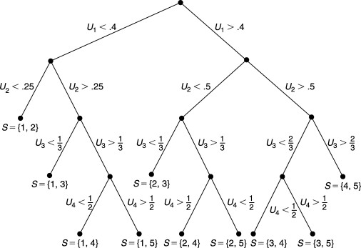
For example, if we want to choose a subset of size k=2 from n=5 elements, the process can be visualized as a decision tree, as shown in Figure 5.5.
 Figure 5.5
Alt text: Tree diagram illustrating the process of selecting a random subset of size 2 from 5 elements using uniform random variables, showing probabilities at each branch and resulting subsets.
Each path to a final position (subset) in the tree has a probability of 1/10, confirming the uniformity of the selection process.
Uniform Distribution Over a Two-Dimensional Region
Another important application of uniform random variables is in defining uniform distributions over regions in multiple dimensions. A random vector (X, Y) is said to have a uniform distribution over a two-dimensional region R if its joint probability density function is constant within R and zero outside R.
Mathematically, the joint density function f(x, y) is given by:
f(x,y) = { c if (x, y) ∈ R
{ 0 otherwise
To find the constant c, we use the property that the integral of the density function over the entire space must be equal to 1:
∫∫R f(x, y) dx dy = 1
∫∫R c dx dy = c × Area of R = 1
Thus, c = 1 / Area of R
For any subregion A within R, the probability that (X, Y) falls into A is:
P{(X, Y) ∈ A} = ∫∫A f(x, y) dx dy = ∫∫A c dx dy = Area of A / Area of R
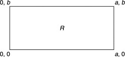
Consider a specific case where R is a rectangle defined by 0 ≤ x ≤ a and 0 ≤ y ≤ b.
 Rectangle Region R
Alt text: Rectangular region R in a two-dimensional plane, defined by bounds 0 to a on the x-axis and 0 to b on the y-axis, illustrating a uniform distribution.
For this rectangular region, the area is a b, and hence c = 1 / (a b). The joint density function is:
f(x,y) = { 1/(a b) if 0 ≤ x ≤ a, 0 ≤ y ≤ b
{ 0 otherwise
In this scenario, interestingly, X and Y are independent uniform random variables. To see this, let’s calculate the cumulative distribution functions (CDFs). For 0 ≤ x ≤ a and 0 ≤ y ≤ b:
P(X ≤ x, Y ≤ y) = ∫x0 ∫y0 f(u, v) dv du = ∫x0 ∫y0 (1/(a b)) dv du = (x y) / (a b)
Now, let’s find the marginal CDFs of X and Y:
P(X ≤ x) = P(X ≤ x, Y ≤ b) = (x b) / (a b) = x/a for 0 ≤ x ≤ a
P(Y ≤ y) = P(X ≤ a, Y ≤ y) = (a y) / (a b) = y/b for 0 ≤ y ≤ b
Since P(X ≤ x, Y ≤ y) = P(X ≤ x) P(Y ≤ y), X and Y are indeed independent, with X being uniformly distributed on (0, a) and Y uniformly distributed on (0, b*).
Conclusion
Uniform random variables are a cornerstone in probability due to their simplicity and wide applicability. From generating random selections to defining distributions over geometric regions, they provide a fundamental building block for more complex probabilistic models and simulations. Understanding uniform random variables is crucial for anyone working in statistics, probability, computer simulation, and related fields. Their equal probability characteristic makes them ideal for scenarios where fairness and unbiased selection are paramount.
