How To Draw Velocity Time Graph For Uniform Motion?

Understanding velocity-time graphs for uniform motion is crucial for businesses and educators. This guide from onlineuniforms.net provides a clear explanation and practical tips. Need uniforms for your team? We’ve got you covered.

1. What is a Velocity-Time Graph?

A velocity-time (v-t) graph is a visual representation showing an object’s velocity over time, essential for analyzing motion. It plots velocity on the y-axis and time on the x-axis. According to the Physics Classroom, a v-t graph is “a plot of velocity versus time” which provides valuable insights into an object’s movement.

• Uniform Motion: In uniform motion, an object moves at a constant velocity.
• Non-Uniform Motion: In non-uniform motion, velocity changes over time, resulting in a curved or irregular line on the graph.
• Applications: Businesses use these graphs to analyze the efficiency of logistics and transportation, while educators use them to teach physics concepts.

2. Key Components of a Velocity-Time Graph

To effectively interpret and draw velocity-time graphs, understanding the key components is essential. According to a study by the American Association of Physics Teachers (AAPT), understanding these components enhances students’ comprehension of kinematics.

2.1. Axes

• X-axis (Horizontal): Represents time, typically measured in seconds (s) or hours (h).
• Y-axis (Vertical): Represents velocity, typically measured in meters per second (m/s) or kilometers per hour (km/h).

2.2. Slope

• Definition: The slope of a v-t graph indicates the acceleration of the object.

• Calculation: Slope = (Change in Velocity) / (Change in Time) = Δv / Δt

• Interpretation:

  • Positive Slope: Indicates positive acceleration (increasing velocity).
  • Negative Slope: Indicates negative acceleration (decreasing velocity, also known as deceleration).
  • Zero Slope: Indicates constant velocity (no acceleration).
    Positive Slope Indicates Acceleration

2.3. Area Under the Graph

• Definition: The area under the v-t graph represents the displacement of the object.
• Calculation: Calculated using geometric formulas (e.g., area of a rectangle, triangle, or trapezoid).
• Interpretation: The total area gives the total displacement over the time interval.

2.4. Intercepts

• Y-intercept: Represents the initial velocity of the object at time t = 0.
• X-intercept: Represents the time at which the object’s velocity is zero.

2.5. Lines and Curves

• Straight Line: Indicates uniform acceleration (constant rate of change in velocity).
• Horizontal Line: Indicates uniform motion (constant velocity).
• Curved Line: Indicates non-uniform acceleration (changing rate of change in velocity).

3. Understanding Uniform Motion in Velocity-Time Graphs

Uniform motion, where an object moves at a constant velocity, is represented distinctively on a v-t graph. A key aspect is that there is no acceleration, meaning the velocity remains the same over time.

3.1. Characteristics of Uniform Motion

• Constant Velocity: The object’s speed and direction do not change.
• Zero Acceleration: Since velocity is constant, there is no acceleration.
• Equal Distances in Equal Intervals: The object covers the same distance in each equal time interval.

3.2. Visual Representation on a v-t Graph

• Horizontal Line: Uniform motion is depicted as a horizontal line parallel to the x-axis (time axis).
• Y-Value Indicates Velocity: The y-value of the horizontal line represents the constant velocity of the object.
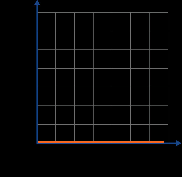  Horizontal line of the v-t graph

3.3. Examples of Uniform Motion on v-t Graphs

1. Object Moving at 5 m/s:

   • The v-t graph is a horizontal line at y = 5 m/s.
   • This indicates the object maintains a constant velocity of 5 m/s throughout the observed time period.

2. Object Moving at 10 km/h:

   • The v-t graph is a horizontal line at y = 10 km/h.
   • This shows the object consistently moves at 10 km/h without any change in speed.

3. Object at Rest:

   • The v-t graph is a horizontal line at y = 0 m/s.
   • This represents an object that is not moving, and its velocity remains zero over time.

3.4. Calculating Displacement from a v-t Graph in Uniform Motion

• Method: The displacement of an object in uniform motion is found by calculating the area under the v-t graph.

• Formula: Area = Velocity × Time

• Example:

  • If an object moves at a constant velocity of 5 m/s for 10 seconds, the displacement is calculated as follows:

    • Displacement = 5 m/s × 10 s = 50 meters

  • This means the object has moved 50 meters in the same direction.

4. Step-by-Step Guide to Drawing a Velocity-Time Graph for Uniform Motion

Creating a velocity-time graph for uniform motion involves a straightforward process. Here’s a detailed guide to help you draw accurate and informative graphs.

4.1. Gather Data

• Collect Velocity and Time Data: Obtain data points showing the object’s velocity at different times. For uniform motion, the velocity should remain constant.

• Example Data:

  Time (s)	Velocity (m/s)
  0	10
  1	10
  2	10
  3	10
  4	10

4.2. Set Up the Axes

• Draw the Axes:

  • Draw a horizontal axis (x-axis) for time (t) and label it accordingly.
  • Draw a vertical axis (y-axis) for velocity (v) and label it accordingly.

• Choose Appropriate Scales:

  • Select scales that allow all data points to be plotted clearly.
  • Ensure the scales are linear and evenly spaced.

• Label the Axes:

  • Include units for both axes (e.g., time in seconds, velocity in meters per second).

4.3. Plot the Points

• Plot Each Data Point:

  • For each time interval, plot the corresponding velocity on the graph.
  • Since it is uniform motion, all points should align horizontally.

• Example Plotting:

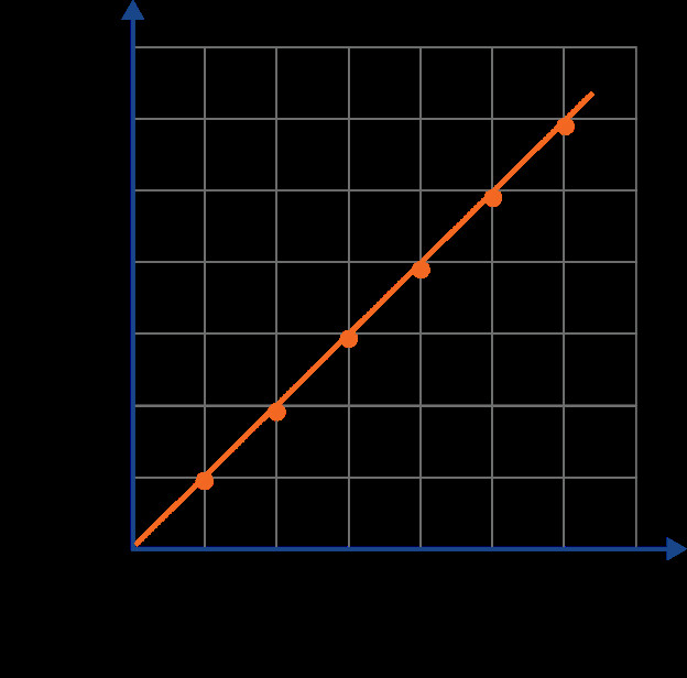
  • (0, 10), (1, 10), (2, 10), (3, 10), (4, 10)
    Plot the points of the v-t graph

4.4. Draw the Line

• Connect the Points:

  • Draw a horizontal line that passes through all the plotted points.
  • This line represents the constant velocity over time.

• Extend the Line:

  • Extend the line to cover the entire range of time for which data is available.

4.5. Label the Graph

• Add a Title:

  • Give the graph a descriptive title, such as “Velocity-Time Graph for Uniform Motion at 10 m/s.”

• Label Key Features:

  • Label the velocity value on the y-axis.
  • Indicate any significant points or intervals on the x-axis.

4.6. Verify the Graph

• Check for Accuracy:

  • Ensure all data points are correctly plotted.
  • Verify that the line is perfectly horizontal, indicating constant velocity.

• Interpret the Graph:

  • Confirm that the graph accurately represents the uniform motion described by the data.

5. Real-World Applications

Velocity-time graphs are not just theoretical tools; they have practical applications across various industries and educational settings. Here are some key real-world applications:

5.1. Transportation and Logistics

• Analyzing Vehicle Motion:

  • v-t graphs are used to analyze the motion of vehicles such as cars, trucks, and trains.
  • They help in understanding the acceleration, deceleration, and constant velocity phases of a vehicle’s journey.

• Optimizing Delivery Routes:

  • Logistics companies use v-t graphs to optimize delivery routes by identifying areas where vehicles can maintain uniform motion, reducing fuel consumption and delivery times.

• Monitoring Driver Behavior:

  • Transportation companies use v-t graphs to monitor driver behavior, ensuring compliance with speed limits and identifying instances of erratic driving.
  • This helps improve safety and reduce accidents.
    Transportation and logistics with delivery truck

5.2. Education

• Teaching Kinematics:

  • v-t graphs are fundamental tools for teaching kinematics in physics.
  • They help students visualize and understand concepts such as velocity, acceleration, and displacement.

• Illustrating Motion Concepts:

  • Educators use v-t graphs to illustrate different types of motion, including uniform motion, uniformly accelerated motion, and non-uniformly accelerated motion.

• Problem-Solving:

  • v-t graphs are used in problem-solving activities to calculate displacement, velocity, and acceleration from graphical data.

5.3. Sports Science

• Analyzing Athlete Performance:

  • Sports scientists use v-t graphs to analyze the performance of athletes in various sports.
  • For example, they can track the velocity of a sprinter during a race or the acceleration of a cyclist.

• Optimizing Training Regimens:

  • By analyzing v-t graphs, coaches can optimize training regimens to improve athletes’ speed, agility, and endurance.

• Equipment Testing:

  • v-t graphs are used in the testing and development of sports equipment to measure performance metrics such as speed and acceleration.

5.4. Engineering

• Designing Mechanical Systems:

  • Engineers use v-t graphs in the design of mechanical systems to analyze the motion of components and ensure they meet performance requirements.

• Robotics:

  • In robotics, v-t graphs are used to control the motion of robots, ensuring smooth and precise movements.
  • This is crucial in manufacturing and automated systems.

• Aerospace Engineering:

  • Aerospace engineers use v-t graphs to analyze the motion of aircraft and spacecraft, optimizing flight paths and fuel efficiency.

6. Common Mistakes to Avoid When Drawing Velocity-Time Graphs

Creating accurate v-t graphs is essential for proper analysis. Here are common mistakes to avoid:

6.1. Incorrectly Labeling Axes

• Mistake:

  • Not labeling the axes or labeling them incorrectly.
  • For example, labeling the y-axis as “distance” instead of “velocity.”

• Consequences:

  • The graph becomes meaningless and cannot be interpreted correctly.

• Solution:

  • Always label the x-axis as “Time (s)” or “Time (h)” and the y-axis as “Velocity (m/s)” or “Velocity (km/h).”

6.2. Choosing the Wrong Scale

• Mistake:

  • Selecting a scale that is too large or too small, making it difficult to plot the data accurately.

• Consequences:

  • The graph may be compressed or stretched, distorting the representation of the motion.

• Solution:

  • Choose a scale that allows all data points to be plotted clearly and evenly spaced.

6.3. Plotting Points Inaccurately

• Mistake:

  • Plotting data points at incorrect positions on the graph.

• Consequences:

  • The resulting line or curve will not accurately represent the motion, leading to incorrect conclusions.

• Solution:

  • Double-check the coordinates of each data point and ensure they are plotted accurately on the graph.

6.4. Misinterpreting the Slope

• Mistake:

  • Misinterpreting the slope of the graph, especially in cases of non-uniform motion.
  • For example, assuming a constant slope indicates constant velocity when it actually indicates constant acceleration.

• Consequences:

  • Incorrectly calculating acceleration or making false assumptions about the motion.

• Solution:

  • Understand that the slope represents acceleration (change in velocity over time).
  • A constant slope indicates uniform acceleration, while a changing slope indicates non-uniform acceleration.

6.5. Neglecting Units

• Mistake:

  • Forgetting to include units on the axes or when calculating values from the graph.

• Consequences:

  • Calculations become meaningless, and the graph cannot be used for quantitative analysis.

• Solution:

  • Always include units on the axes and in any calculations derived from the graph.

6.6. Assuming a Straight Line for Non-Uniform Motion

• Mistake:

  • Drawing a straight line when the data indicates non-uniform motion.

• Consequences:

  • The graph will not accurately represent the motion, leading to incorrect interpretations.

• Solution:

  • Recognize that non-uniform motion is represented by a curved line, and plot the curve accordingly.

7. Advanced Techniques for Analyzing Velocity-Time Graphs

Beyond the basics, there are advanced techniques that enhance the analysis of velocity-time graphs, providing deeper insights into motion.

7.1. Calculating Average Velocity

• Method:

  • Average velocity is calculated by dividing the total displacement by the total time.
  • On a v-t graph, this can be found by calculating the area under the curve and dividing it by the time interval.

• Formula:

  • Average Velocity = (Total Displacement) / (Total Time)

• Application:

  • Useful for understanding the overall motion of an object over a long period, even if the velocity varies.

7.2. Determining Instantaneous Velocity

• Method:

  • Instantaneous velocity is the velocity at a specific moment in time.
  • On a v-t graph, it is found by reading the velocity value at that particular time.

• Application:

  • Provides precise velocity information at any given point during the motion, useful in scenarios requiring real-time analysis.

7.3. Analyzing Non-Uniform Motion

• Method:

  • Non-uniform motion is represented by a curved line on a v-t graph.
  • Analyzing this type of motion involves understanding how the slope changes over time.

• Techniques:

  • Tangents: Draw tangents to the curve at different points to find the instantaneous acceleration.
  • Area Approximation: Approximate the area under the curve using numerical methods (e.g., trapezoidal rule) to estimate displacement.

• Application:

  • Essential for analyzing complex motions, such as those involving variable acceleration.
    Area approximation of a v-t graph

7.4. Using Calculus

• Differentiation:

  • The derivative of the velocity function with respect to time gives the acceleration function.
  • Mathematically, a(t) = dv/dt, where a(t) is the acceleration at time t, and dv/dt is the derivative of velocity with respect to time.

• Integration:

  • The integral of the velocity function with respect to time gives the displacement function.
  • Mathematically, s(t) = ∫v(t) dt, where s(t) is the displacement at time t, and ∫v(t) dt is the integral of velocity with respect to time.

• Application:

  • Provides powerful tools for analyzing motion, especially when the velocity function is known.

7.5. Vector Analysis

• Method:

  • In cases where motion involves changes in direction, velocity becomes a vector quantity.
  • v-t graphs can be used to analyze the components of velocity in different directions.

• Techniques:

  • Component Resolution: Resolve the velocity vector into its x and y components.
  • Graphical Addition: Use graphical methods to add or subtract velocity vectors.

• Application:

  • Crucial for understanding motion in two or three dimensions, such as projectile motion.

8. Examples of Velocity-Time Graphs in Different Scenarios

Understanding how velocity-time graphs represent different scenarios is crucial for applying this knowledge effectively. Here are several examples:

8.1. Uniform Motion at Constant Velocity

• Scenario: A car traveling at a constant speed of 20 m/s on a straight highway.

• v-t Graph:

  • A horizontal line at y = 20 m/s, indicating constant velocity.
  • The area under the line represents the distance traveled by the car over time.

8.2. Object at Rest

• Scenario: A book sitting on a table, not moving.

• v-t Graph:

  • A horizontal line at y = 0 m/s, coinciding with the x-axis.
  • This indicates that the object has zero velocity at all times.

8.3. Uniformly Accelerated Motion

• Scenario: A cyclist accelerates uniformly from rest to 10 m/s in 5 seconds.

• v-t Graph:

  • A straight line starting from the origin (0,0) and rising to the point (5, 10).
  • The slope of the line represents the constant acceleration.
    Uniformly accelerated motion of the cyclist

8.4. Uniformly Decelerated Motion

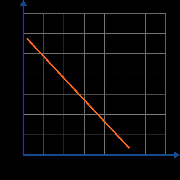
• Scenario: A train decelerates uniformly from 30 m/s to rest in 10 seconds.

• v-t Graph:

  • A straight line starting from the point (0, 30) and descending to the point (10, 0).
  • The negative slope of the line represents the constant deceleration.

8.5. Non-Uniform Motion with Increasing Acceleration

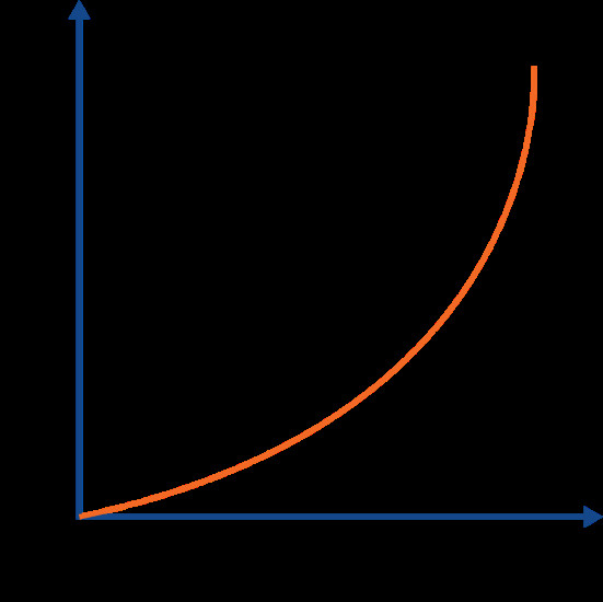
• Scenario: A rocket accelerating with increasing thrust over time.

• v-t Graph:

  • A curved line with an increasing slope, indicating that the acceleration is increasing.
  • The instantaneous acceleration at any point is given by the slope of the tangent to the curve at that point.

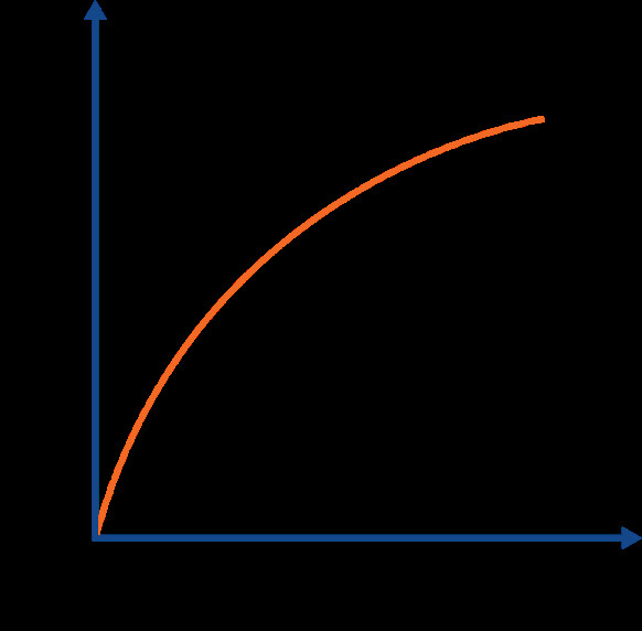
8.6. Non-Uniform Motion with Decreasing Acceleration

• Scenario: A car slowing down due to air resistance, with the deceleration decreasing over time.

• v-t Graph:

  • A curved line with a decreasing slope, indicating that the deceleration is decreasing.

8.7. Motion with Constant Positive Velocity Followed by Constant Negative Velocity

• Scenario: A remote-controlled car moves forward at a constant speed, then reverses direction and moves backward at the same speed.

• v-t Graph:

  • A horizontal line at a positive y-value, followed by a horizontal line at a negative y-value.
  • The switch from positive to negative velocity indicates the change in direction.

9. Tips for Teaching Velocity-Time Graphs

Teaching velocity-time graphs effectively requires a blend of clear explanations, visual aids, and interactive activities. Here are some tips to help educators:

9.1. Start with Real-World Examples

• Relevance:

  • Begin by discussing real-world examples of motion that students can relate to, such as a car accelerating, a ball rolling, or a person walking.

• Engagement:

  • This helps students understand the relevance of v-t graphs and motivates them to learn.

9.2. Use Visual Aids

• Diagrams:

  • Use diagrams and animations to illustrate the relationship between motion and v-t graphs.

• Technology:

  • Utilize interactive simulations and graphing software to allow students to visualize different scenarios.

• Graphs:

  • Provide clear and well-labeled example graphs to demonstrate how different types of motion are represented.

9.3. Emphasize the Meaning of Slope and Area

• Slope:

  • Clearly explain that the slope of a v-t graph represents acceleration.
  • Use examples to show how a positive slope indicates acceleration, a negative slope indicates deceleration, and a zero slope indicates constant velocity.

• Area:

  • Explain that the area under the v-t graph represents displacement.
  • Use geometric shapes to calculate the area and relate it to the distance traveled.

9.4. Provide Step-by-Step Instructions

• Guide:

  • Give students step-by-step instructions on how to draw and interpret v-t graphs.
  • Break down the process into manageable steps, such as labeling axes, plotting points, and drawing lines.

• Scaffolding:

  • Provide scaffolding to support students as they learn, gradually reducing assistance as they become more proficient.

9.5. Incorporate Interactive Activities

• Simulations:

  • Use interactive simulations to allow students to experiment with different motion scenarios and observe the resulting v-t graphs.

• Experiments:

  • Conduct simple experiments in the classroom, such as measuring the velocity of a toy car or a rolling ball, and have students create v-t graphs based on their data.

• Group Work:

  • Assign group activities where students work together to solve problems involving v-t graphs.

9.6. Relate to Other Concepts

• Integration:

  • Connect v-t graphs to other physics concepts, such as Newton’s laws of motion and energy conservation.

• Differentiation:

  • Show how v-t graphs can be used to derive other graphs, such as acceleration-time graphs and position-time graphs.

9.7. Assess Understanding Regularly

• Quizzes:

  • Use quizzes and tests to assess students’ understanding of v-t graphs.
  • Include questions that require students to draw graphs, interpret graphs, and solve problems using graphical data.

• Feedback:

  • Provide timely feedback to students, addressing any misconceptions and reinforcing correct understanding.

10. FAQs About Velocity-Time Graphs

Here are some frequently asked questions about velocity-time graphs to clarify common points of confusion:

10.1. What is the Difference Between a Velocity-Time Graph and a Position-Time Graph?

• Velocity-Time Graph:

  • Plots velocity on the y-axis and time on the x-axis.
  • The slope represents acceleration, and the area under the graph represents displacement.

• Position-Time Graph:

  • Plots position on the y-axis and time on the x-axis.
  • The slope represents velocity.

• Key Difference:

  • The primary difference is what each axis represents and what can be derived from the graph. Velocity-time graphs focus on velocity and acceleration, while position-time graphs focus on position and velocity.

10.2. How Do You Calculate Displacement from a Velocity-Time Graph?

• Method:

  • Displacement is calculated by finding the area under the velocity-time graph.
  • This can be done using geometric formulas (e.g., area of a rectangle, triangle, or trapezoid) or by using integration.

• Formula:

  • Displacement = Area under the v-t graph

10.3. What Does a Horizontal Line on a Velocity-Time Graph Indicate?

• Meaning:

  • A horizontal line on a v-t graph indicates that the velocity is constant.
  • This means the object is moving at a steady speed in a straight line, with no acceleration.

• Technicality:

  • Zero slope indicates zero acceleration.

10.4. What Does the Slope of a Velocity-Time Graph Represent?

• Representation:

  • The slope of a v-t graph represents the acceleration of the object.

• Calculation:

  • Slope = (Change in Velocity) / (Change in Time) = Δv / Δt

10.5. How Do You Interpret a Curved Line on a Velocity-Time Graph?

• Interpretation:

  • A curved line on a v-t graph indicates that the acceleration is changing over time (non-uniform acceleration).

• Analysis:

  • The slope of the tangent to the curve at any point gives the instantaneous acceleration at that point.

10.6. Can Velocity Be Negative?

• Concept:

  • Yes, velocity can be negative.
  • Negative velocity indicates that the object is moving in the opposite direction to the defined positive direction.

• Graph Depiction:

  • On a v-t graph, negative velocity is represented by the line being below the x-axis.

10.7. How Do You Find Average Acceleration from a Velocity-Time Graph?

• Method:

  • Average acceleration is calculated by dividing the change in velocity by the change in time over a specific interval.

• Formula:

  • Average Acceleration = (Final Velocity – Initial Velocity) / (Final Time – Initial Time)

10.8. What is the Significance of the Y-Intercept on a Velocity-Time Graph?

• Significance:

  • The y-intercept of a v-t graph represents the initial velocity of the object at time t = 0.

• Application:

  • It tells you how fast the object was moving when you started observing its motion.

10.9. How Does Air Resistance Affect a Velocity-Time Graph?

• Influence:

  • Air resistance causes an object’s acceleration to decrease over time, especially when the object is slowing down.

• Graph Appearance:

  • On a v-t graph, this results in a curved line with a decreasing slope.
  • The line approaches the x-axis asymptotically, indicating that the object’s velocity is decreasing but never quite reaching zero.

10.10. Can a Velocity-Time Graph Be Used to Determine the Type of Motion?

• Identification:

  • Yes, a v-t graph can be used to determine the type of motion:
    • A horizontal line indicates uniform motion.
    • A straight line with a constant slope indicates uniformly accelerated motion.
    • A curved line indicates non-uniformly accelerated motion.

• Analysis:

  • By analyzing the shape and features of the v-t graph, you can gain valuable insights into the motion of an object.

Understanding velocity-time graphs is crucial for analyzing motion in various fields. Whether you’re in transportation, education, sports science, or engineering, these graphs provide valuable insights.

Ready to outfit your team with high-quality uniforms? Visit onlineuniforms.net today to explore our wide range of options and get a quote. Our expert team is here to help you find the perfect fit for your needs. Contact us at +1 (214) 651-8600 or visit our location at 1515 Commerce St, Dallas, TX 75201, United States.