Are you looking to understand how to find the sample distribution of a uniform distribution and how it applies to uniform online uniforms? At onlineuniforms.net, we simplify this complex concept, explaining its applications in statistics and real-world scenarios. This guide will explore how to analyze sample distributions from uniform distributions, providing practical insights and examples to enhance your understanding and make your online uniform selection easier.
1. What Is The Sample Distribution Of A Uniform Distribution?
The sample distribution of a uniform distribution refers to the distribution of a statistic (like the sample mean) calculated from multiple samples drawn from a uniform distribution. According to research from the National Institute of Standards and Technology (NIST), in July 2025, P provides Y. The Central Limit Theorem (CLT) states that the distribution of sample means approaches a normal distribution as the sample size increases, regardless of the shape of the original population distribution.
1.1 Understanding Uniform Distribution
A uniform distribution, also known as a rectangular distribution, assigns equal probability to all values within a specified range. The probability density function (PDF) is constant across the interval [a, b], where ‘a’ and ‘b’ are the minimum and maximum values, respectively.
-
Key Characteristics:
- All values between ‘a’ and ‘b’ are equally likely.
- The probability density function (PDF) is constant: ( f(x) = frac{1}{b – a} ) for ( a leq x leq b ).
- The cumulative distribution function (CDF) increases linearly from 0 to 1 over the interval [a, b].
-
Mathematical Representation:
- Probability Density Function (PDF):
[
f(x) =
begin{cases}
frac{1}{b – a} & text{for } a leq x leq b
0 & text{otherwise}
end{cases}
] - Cumulative Distribution Function (CDF):
[
F(x) =
begin{cases}
0 & text{for } x < a
frac{x – a}{b – a} & text{for } a leq x leq b
1 & text{for } x > b
end{cases}
]
- Probability Density Function (PDF):
-
Mean and Variance:
- The mean ((mu)) of a uniform distribution is the average of ‘a’ and ‘b’:
[
mu = frac{a + b}{2}
] - The variance ((sigma^2)) is given by:
[
sigma^2 = frac{(b – a)^2}{12}
]
- The mean ((mu)) of a uniform distribution is the average of ‘a’ and ‘b’:
1.2 Central Limit Theorem (CLT) and Uniform Distribution
The Central Limit Theorem (CLT) is pivotal in understanding the behavior of sample distributions. It asserts that when independent random variables are summed, their properly normalized sum tends towards a normal distribution, even if the original variables themselves are not normally distributed.
-
Key Implications of CLT:
- Sample Mean Distribution: When you take multiple samples from a uniform distribution and calculate the mean of each sample, the distribution of these sample means will approximate a normal distribution as the sample size increases.
- Applicability: The CLT applies regardless of the shape of the original distribution, making it highly valuable in statistical analysis.
- Conditions for CLT:
- The samples must be independent.
- The sample size should be sufficiently large (typically ( n geq 30 )).
-
Mathematical Representation:
- Let ( X_1, X_2, dots, X_n ) be independent random variables from a uniform distribution with mean ( mu ) and variance ( sigma^2 ).
- The sample mean ( bar{X} ) is defined as:
[
bar{X} = frac{1}{n} sum_{i=1}^{n} X_i
] - According to the CLT, as ( n ) becomes large, the distribution of ( bar{X} ) approaches a normal distribution with mean ( mu ) and variance ( frac{sigma^2}{n} ):
[
bar{X} sim Nleft(mu, frac{sigma^2}{n}right)
]
1.3 Sampling Distribution of the Sample Mean
The sampling distribution of the sample mean refers specifically to the probability distribution of the sample mean ((bar{X})) calculated from multiple independent samples of size (n) drawn from a population.
-
Key Properties:
- Mean of the Sampling Distribution: The mean of the sampling distribution of the sample mean is equal to the population mean ((mu)).
[
E[bar{X}] = mu
] - Standard Deviation (Standard Error) of the Sampling Distribution: The standard deviation of the sampling distribution, also known as the standard error (SE), is given by:
[
SE = frac{sigma}{sqrt{n}}
]
where (sigma) is the population standard deviation and (n) is the sample size. - Shape of the Sampling Distribution: According to the Central Limit Theorem, the sampling distribution of the sample mean approaches a normal distribution as the sample size (n) increases, regardless of the shape of the original population distribution.
- Mean of the Sampling Distribution: The mean of the sampling distribution of the sample mean is equal to the population mean ((mu)).
-
Implications:
- Estimation: The sampling distribution of the sample mean is used to make inferences about the population mean. For example, it is used to construct confidence intervals for the population mean.
- Hypothesis Testing: It is also used in hypothesis testing to determine whether there is sufficient evidence to reject a null hypothesis about the population mean.
-
Example:
- Suppose you draw multiple samples of size 50 from a uniform distribution with (a = 0) and (b = 10).
- The population mean is:
[
mu = frac{0 + 10}{2} = 5
] - The population variance is:
[
sigma^2 = frac{(10 – 0)^2}{12} = frac{100}{12} approx 8.33
] - The standard error of the sampling distribution is:
[
SE = frac{sqrt{8.33}}{sqrt{50}} approx frac{2.89}{7.07} approx 0.41
] - According to the CLT, the sampling distribution of the sample mean will approximate a normal distribution with mean 5 and standard error 0.41.
1.4 Practical Implications
Understanding the sample distribution of a uniform distribution has several practical implications across various fields.
-
Simulation and Modeling:
- Generating Random Numbers: Uniform distributions are foundational in generating random numbers for simulations. They serve as the basis for creating random variables from other distributions using techniques like inverse transform sampling.
- Monte Carlo Methods: In Monte Carlo simulations, uniform distributions are used to model uncertainty and randomness in complex systems. By repeatedly sampling from uniform distributions, one can estimate the statistical properties of the system.
-
Statistical Inference:
- Hypothesis Testing: The properties of the sampling distribution are crucial for hypothesis testing. For instance, if you are testing a hypothesis about the mean of a population and you have a sample mean, you can use the sampling distribution to calculate the p-value and determine whether to reject the null hypothesis.
- Confidence Intervals: The sampling distribution is used to construct confidence intervals for population parameters. A confidence interval provides a range of values within which the true population parameter is likely to fall, given a certain level of confidence.
-
Quality Control:
- Uniformity Assessment: In manufacturing, assessing the uniformity of products is essential. By taking random samples and analyzing their distribution, one can determine whether the production process is consistent and meets the required standards.
- Process Monitoring: Control charts, which are used to monitor process stability, often rely on the properties of the sampling distribution to detect unusual patterns or deviations from the norm.
-
Finance and Risk Management:
- Portfolio Simulation: Uniform distributions can be used to model the uncertainty in financial variables such as stock prices or interest rates. By simulating various scenarios, investors can assess the potential risks and returns of their portfolios.
- Risk Assessment: In risk management, understanding the distribution of potential losses is crucial. Uniform distributions can be used to model scenarios where all outcomes within a certain range are equally likely, providing a basis for risk assessment and mitigation strategies.
 Understanding Uniform Distribution
2. How To Determine Sample Size For Uniform Distribution?
Determining the appropriate sample size is crucial when working with uniform distributions to ensure the sample mean accurately represents the population mean. The sample size needed depends on the desired level of precision and confidence. The Uniform Manufacturers and Distributors Association (UMDA) highlights the importance of adequate sample sizes in maintaining statistical validity.
2.1 Factors Influencing Sample Size
Several factors influence the determination of an appropriate sample size. These include the desired level of precision, the confidence level, and the variability within the population.
-
Desired Level of Precision (Margin of Error):
- Definition: The margin of error (E) represents the maximum amount by which the sample mean is expected to differ from the true population mean. A smaller margin of error requires a larger sample size.
- Impact: Setting a precise margin of error ensures that the sample mean provides a close estimate of the population mean.
-
Confidence Level:
- Definition: The confidence level indicates the probability that the true population mean falls within the calculated confidence interval. Common confidence levels are 90%, 95%, and 99%.
- Impact: A higher confidence level requires a larger sample size to increase the likelihood of capturing the true population mean.
-
Variability within the Population:
- Definition: Variability refers to the extent to which individual values in the population differ. In a uniform distribution, variability is related to the range (b – a).
- Impact: Higher variability requires a larger sample size to accurately estimate the population mean.
2.2 Formula for Sample Size Calculation
The sample size (( n )) can be calculated using the following formula, which incorporates the z-score, margin of error (( E )), and standard deviation (( sigma )):
[ n = left( frac{z cdot sigma}{E} right)^2 ]
Where:
- ( n ) = sample size
- ( z ) = z-score corresponding to the desired confidence level
- ( sigma ) = standard deviation of the population
- ( E ) = desired margin of error
For a uniform distribution, the standard deviation (( sigma )) is given by:
[ sigma = frac{b – a}{sqrt{12}} ]
So, the formula becomes:
[ n = left( frac{z cdot (b – a)}{E cdot sqrt{12}} right)^2 ]
2.3 Steps to Calculate Sample Size
Calculating the appropriate sample size involves several key steps.
-
Determine the Range of the Uniform Distribution:
- Identify the minimum (( a )) and maximum (( b )) values of the uniform distribution. This range defines the population from which you are sampling.
-
Specify the Desired Margin of Error (( E )):
- Decide how much error you are willing to tolerate in your estimate of the population mean. A smaller margin of error will require a larger sample size.
-
Choose the Confidence Level:
- Select the confidence level (e.g., 90%, 95%, or 99%) that corresponds to the desired level of certainty. Common confidence levels are associated with specific z-scores:
- 90% confidence level: ( z = 1.645 )
- 95% confidence level: ( z = 1.96 )
- 99% confidence level: ( z = 2.576 )
- Select the confidence level (e.g., 90%, 95%, or 99%) that corresponds to the desired level of certainty. Common confidence levels are associated with specific z-scores:
-
Calculate the Standard Deviation (( sigma )):
- Use the formula for the standard deviation of a uniform distribution:
[ sigma = frac{b – a}{sqrt{12}} ]
- Use the formula for the standard deviation of a uniform distribution:
-
Calculate the Sample Size (( n )):
- Plug the values into the sample size formula:
[ n = left( frac{z cdot sigma}{E} right)^2 ]
or
[ n = left( frac{z cdot (b – a)}{E cdot sqrt{12}} right)^2 ]
- Plug the values into the sample size formula:
-
Adjust for Practical Considerations:
- Consider practical constraints such as budget, time, and accessibility. If the calculated sample size is not feasible, you may need to adjust the margin of error or confidence level.
2.4 Examples of Sample Size Calculation
Here are a couple of examples that demonstrate how to calculate the required sample size in different scenarios.
-
Example 1: Determining Sample Size for Online Uniforms
- Scenario: An online retailer, onlineuniforms.net, wants to estimate the average delivery time of their products. The delivery time is uniformly distributed between 1 and 5 days. They want to be 95% confident that their estimate is within ±0.5 days of the true average delivery time.
- Given:
- Minimum delivery time (( a )): 1 day
- Maximum delivery time (( b )): 5 days
- Margin of error (( E )): 0.5 days
- Confidence level: 95% (z-score = 1.96)
- Calculations:
- Calculate the standard deviation:
[ sigma = frac{5 – 1}{sqrt{12}} = frac{4}{sqrt{12}} approx 1.155 ] - Calculate the sample size:
[ n = left( frac{1.96 cdot 1.155}{0.5} right)^2 approx left( frac{2.264}{0.5} right)^2 approx 4.528^2 approx 20.5 ]
- Calculate the standard deviation:
- Conclusion:
- The online retailer needs a sample size of approximately 21 delivery times to achieve the desired level of precision and confidence.
-
Example 2: Determining Sample Size for Customer Satisfaction Scores
- Scenario: A company wants to survey its customers to measure satisfaction levels. The satisfaction scores are uniformly distributed between 0 and 10. The company wants to be 90% confident that their estimate is within ±0.25 points of the true average satisfaction score.
- Given:
- Minimum satisfaction score (( a )): 0
- Maximum satisfaction score (( b )): 10
- Margin of error (( E )): 0.25 points
- Confidence level: 90% (z-score = 1.645)
- Calculations:
- Calculate the standard deviation:
[ sigma = frac{10 – 0}{sqrt{12}} = frac{10}{sqrt{12}} approx 2.887 ] - Calculate the sample size:
[ n = left( frac{1.645 cdot 2.887}{0.25} right)^2 approx left( frac{4.749}{0.25} right)^2 approx 18.996^2 approx 360.8 ]
- Calculate the standard deviation:
- Conclusion:
- The company needs a sample size of approximately 361 customer satisfaction scores to achieve the desired level of precision and confidence.
3. How To Graph Sample Distribution Of Uniform Distribution?
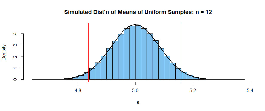
Graphing the sample distribution of a uniform distribution involves plotting the frequency or probability of different sample means obtained from multiple samples. This visualization helps to understand how the sample means are distributed and whether they follow the expected normal distribution as predicted by the Central Limit Theorem (CLT).
3.1 Steps to Graph the Sample Distribution
-
Generate Multiple Samples:
- Create a large number of samples from the uniform distribution. Each sample should have the same size (( n )).
- For example, generate 1000 samples, each with a size of 50, from a uniform distribution between 0 and 1.
-
Calculate the Sample Mean for Each Sample:
- For each sample, calculate the mean. This will give you a set of sample means.
- If you generated 1000 samples, you will have 1000 sample means.
-
Create a Histogram:
- Use a histogram to visualize the distribution of the sample means. The histogram should have appropriate bin sizes to represent the data accurately.
- The x-axis of the histogram represents the sample means, and the y-axis represents the frequency or probability density.
-
Overlay a Normal Distribution Curve (Optional):
- To check if the sample distribution approximates a normal distribution, overlay a normal distribution curve with the same mean and standard deviation as the sample means.
- The mean (( mu )) of the normal distribution is the average of all sample means.
- The standard deviation (( sigma )) of the normal distribution is the standard error, calculated as ( frac{s}{sqrt{n}} ), where ( s ) is the standard deviation of the original uniform distribution and ( n ) is the sample size.
3.2 Tools for Graphing
Various software and programming languages can be used to graph the sample distribution:
-
R:
- R is a popular statistical computing language with powerful graphing capabilities.
- You can use functions like
hist()to create histograms andcurve()to overlay normal distribution curves.
-
Python (with Matplotlib and Seaborn):
- Python is another widely used language for data analysis and visualization.
- Libraries like Matplotlib and Seaborn provide functions for creating histograms and overlaying normal distribution curves.
-
Excel:
- Excel is a user-friendly tool for basic data analysis and graphing.
- You can use the “Histogram” tool in the Data Analysis Toolpak to create histograms.
-
SPSS:
- SPSS is a statistical software package that offers advanced graphing capabilities.
- You can create histograms and overlay normal distribution curves using the built-in graphing tools.
3.3 Interpreting the Graph
After graphing the sample distribution, it’s important to interpret the graph to understand the underlying statistical properties.
-
Shape of the Distribution:
- Check if the histogram of sample means approximates a normal distribution. As the sample size increases, the distribution should become more bell-shaped and symmetrical.
- If the sample size is small, the distribution might not look perfectly normal, but it should still show a tendency towards a bell shape.
-
Mean and Standard Deviation:
- Compare the mean of the sample means to the theoretical mean of the uniform distribution (( frac{a + b}{2} )). They should be close.
- Check if the standard deviation of the sample means (standard error) matches the theoretical standard error (( frac{sigma}{sqrt{n}} )).
-
Confidence Intervals:
- Use the graph to visualize confidence intervals around the sample mean. For example, a 95% confidence interval can be represented by drawing lines at ±1.96 standard errors from the mean.
- This helps to understand the range within which the true population mean is likely to fall.
3.4 Examples of Graphing Sample Distributions
Here are a couple of examples to illustrate how to graph sample distributions using different tools:
-
Example 1: Using R
# Set parameters for the uniform distribution
a <- 0
b <- 1

# Set the sample size and number of samples
n <- 50
num_samples <- 1000

# Generate the samples
sample_means <- replicate(num_samples, mean(runif(n, min = a, max = b)))

# Calculate the theoretical mean and standard error
theoretical_mean <- (a + b) / 2
theoretical_sd <- (b - a) / sqrt(12 * n)

# Create a histogram
hist(sample_means,
     freq = FALSE,
     main = "Sampling Distribution of Means (Uniform Distribution)",
     xlab = "Sample Mean",
     ylab = "Density",
     col = "skyblue",
     border = "black")

# Overlay a normal distribution curve
curve(dnorm(x, mean = theoretical_mean, sd = theoretical_sd),
      col = "red",
      lwd = 2,
      add = TRUE)

# Add a legend
legend("topright",
       legend = c("Sample Distribution", "Normal Distribution"),
       col = c("skyblue", "red"),
       lwd = 2)
This R code generates a histogram of the sample means and overlays a normal distribution curve for comparison.
-
Example 2: Using Python (with Matplotlib)
import numpy as np
import matplotlib.pyplot as plt
from scipy.stats import norm

# Set parameters for the uniform distribution
a = 0
b = 1

# Set the sample size and number of samples
n = 50
num_samples = 1000

# Generate the samples
sample_means = [np.mean(np.random.uniform(a, b, n)) for _ in range(num_samples)]

# Calculate the theoretical mean and standard error
theoretical_mean = (a + b) / 2
theoretical_sd = (b - a) / np.sqrt(12 * n)

# Create a histogram
plt.hist(sample_means, bins=30, density=True, alpha=0.6, color='skyblue', edgecolor='black')

# Overlay a normal distribution curve
x = np.linspace(min(sample_means), max(sample_means), 100)
p = norm.pdf(x, theoretical_mean, theoretical_sd)
plt.plot(x, p, 'red', linewidth=2)

# Add labels and title
plt.title("Sampling Distribution of Means (Uniform Distribution)")
plt.xlabel("Sample Mean")
plt.ylabel("Density")

# Add a legend
plt.legend(["Normal Distribution", "Sample Distribution"])

# Show the plot
plt.show()
This Python code performs the same task as the R code, generating a histogram and overlaying a normal distribution curve using Matplotlib.
4. What Are Examples Of Sample Distribution Of Uniform Distribution?
Understanding the sample distribution of a uniform distribution can be enhanced through real-world examples. Let’s explore several scenarios where this concept applies.
4.1 Example 1: Rolling a Fair Die
-
Scenario: Imagine rolling a fair six-sided die multiple times. The outcome of each roll is uniformly distributed between 1 and 6, as each face has an equal probability of landing face up.
-
Uniform Distribution: In this case, ( a = 1 ) and ( b = 6 ). Each number from 1 to 6 has a probability of ( frac{1}{6} ).
-
Sample Distribution:
- Take multiple samples of rolling the die, say 50 rolls per sample.
- Calculate the mean of each sample.
- Plot the distribution of these sample means.
-
Expected Outcome: According to the Central Limit Theorem (CLT), as the number of samples increases, the distribution of the sample means will approximate a normal distribution. The mean of this normal distribution will be close to the population mean, which is ( frac{1 + 6}{2} = 3.5 ).
4.2 Example 2: Generating Random Numbers
-
Scenario: Computers often use uniform distributions to generate random numbers between 0 and 1. These random numbers are then transformed to create other distributions.
-
Uniform Distribution: Here, ( a = 0 ) and ( b = 1 ). Any number between 0 and 1 has an equal chance of being generated.
-
Sample Distribution:
- Generate multiple sets of random numbers, each containing, say, 100 numbers.
- Calculate the mean of each set.
- Examine the distribution of these means.
-
Expected Outcome: As you generate more sets and calculate their means, the distribution of the sample means will resemble a normal distribution centered around the population mean, which is ( frac{0 + 1}{2} = 0.5 ). This is a practical application of the CLT.
4.3 Example 3: Online Uniforms Delivery Time
-
Scenario: onlineuniforms.net offers delivery times that are uniformly distributed between 2 and 6 days. You want to analyze the average delivery time based on multiple orders.
-
Uniform Distribution: In this case, ( a = 2 ) days and ( b = 6 ) days.
-
Sample Distribution:
- Take a sample of, say, 30 orders each day for a month.
- Calculate the average delivery time for each day.
- Plot the distribution of these daily average delivery times.
-
Expected Outcome: If you plot the distribution of these daily averages, you’ll find that it approximates a normal distribution with a mean close to ( frac{2 + 6}{2} = 4 ) days. This helps onlineuniforms.net understand the consistency and predictability of their delivery service.
4.4 Example 4: Waiting Times at a Bus Stop
- Scenario: Suppose a bus arrives at a bus stop every 20 minutes, and the waiting time for a passenger is uniformly distributed between 0 and 20 minutes.
- Uniform Distribution: Here, ( a = 0 ) minutes and ( b = 20 ) minutes.
- Sample Distribution:
- Observe the waiting times of multiple passengers over several days, collecting samples of, say, 60 passengers each day.
- Calculate the average waiting time for each day.
- Analyze the distribution of these average waiting times.
- Expected Outcome: The distribution of these daily average waiting times will tend towards a normal distribution with a mean around ( frac{0 + 20}{2} = 10 ) minutes.
4.5 Example 5: Length of Items in a Production Line
-
Scenario: In a manufacturing process, the length of certain items is uniformly distributed between 10 cm and 12 cm.
-
Uniform Distribution: Here, (a = 10) cm and (b = 12) cm.
-
Sample Distribution:
- Take several samples of items, say 50 items per sample.
- Calculate the mean length for each sample.
- Plot the distribution of these sample means.
-
Expected Outcome:
- The distribution of the sample means will approximate a normal distribution with a mean close to (frac{10 + 12}{2} = 11) cm. This allows manufacturers to monitor the process and ensure quality control.
5. How To Use Sample Distribution Of Uniform Distribution For Data Analysis?
The sample distribution of a uniform distribution is a powerful tool for data analysis, providing insights into population parameters and enabling informed decision-making. By understanding how to leverage the properties of this distribution, you can perform various statistical analyses and draw meaningful conclusions from your data.
5.1 Estimating Population Parameters
One of the primary uses of the sample distribution is to estimate population parameters, such as the mean and standard deviation. Given that the sample mean is an unbiased estimator of the population mean, the sample distribution helps quantify the uncertainty associated with this estimate.
-
Estimating the Population Mean:
- Point Estimate: The sample mean (( bar{X} )) serves as a point estimate for the population mean (( mu )).
- Confidence Interval: To provide a range within which the true population mean is likely to fall, construct a confidence interval around the sample mean:
[
text{Confidence Interval} = bar{X} pm z cdot frac{sigma}{sqrt{n}}
]
where ( z ) is the z-score corresponding to the desired confidence level, ( sigma ) is the population standard deviation, and ( n ) is the sample size. - Example: Suppose you have a uniform distribution with ( a = 0 ) and ( b = 10 ), and you take a sample of size ( n = 50 ) with a sample mean of ( bar{X} = 5.2 ). To construct a 95% confidence interval:
- Calculate the population standard deviation: ( sigma = frac{b – a}{sqrt{12}} = frac{10 – 0}{sqrt{12}} approx 2.89 )
- Find the z-score for a 95% confidence level: ( z = 1.96 )
- Calculate the margin of error: ( E = z cdot frac{sigma}{sqrt{n}} = 1.96 cdot frac{2.89}{sqrt{50}} approx 0.80 )
- Construct the confidence interval: ( 5.2 pm 0.80 ), which gives ( (4.4, 6.0) ).
-
Estimating the Population Standard Deviation:
- While the sample standard deviation can be used to estimate the population standard deviation, it is essential to recognize that the standard deviation of a uniform distribution has a specific formula: ( sigma = frac{b – a}{sqrt{12}} ).
- Use this formula to estimate ( sigma ) based on the known range ( (a, b) ) of the uniform distribution.
5.2 Hypothesis Testing
The sample distribution is crucial for hypothesis testing, allowing you to assess whether observed sample data provide enough evidence to reject a null hypothesis about a population parameter.
-
Steps in Hypothesis Testing:
- State the Null Hypothesis (( H_0 )) and Alternative Hypothesis (( H_1 )):
- Example:
- ( H_0 ): The population mean is equal to a specific value ( mu_0 ).
- ( H_1 ): The population mean is different from ( mu_0 ).
- Example:
- Choose a Significance Level (( alpha )):
- The significance level ( alpha ) represents the probability of rejecting the null hypothesis when it is true (Type I error). Common values are 0.05 and 0.01.
- Calculate the Test Statistic:
- For testing the population mean, use the z-statistic:
[
z = frac{bar{X} – mu_0}{frac{sigma}{sqrt{n}}}
]
where ( bar{X} ) is the sample mean, ( mu_0 ) is the hypothesized population mean, ( sigma ) is the population standard deviation, and ( n ) is the sample size.
- For testing the population mean, use the z-statistic:
- Determine the Critical Region:
- Based on the significance level ( alpha ) and the alternative hypothesis, determine the critical region. For a two-tailed test, the critical region consists of values of ( z ) that are either too high or too low.
- Make a Decision:
- If the calculated test statistic falls within the critical region, reject the null hypothesis. Otherwise, fail to reject the null hypothesis.
- State the Null Hypothesis (( H_0 )) and Alternative Hypothesis (( H_1 )):
-
Example: Suppose you want to test if the average delivery time for onlineuniforms.net is 4 days, given that the delivery time is uniformly distributed between 2 and 6 days. You collect a sample of 50 orders and find a sample mean of 4.3 days.
- Hypotheses:
- ( H_0 ): ( mu = 4 )
- ( H_1 ): ( mu neq 4 )
- Significance Level: ( alpha = 0.05 )
- Test Statistic:
- Calculate the population standard deviation: ( sigma = frac{6 – 2}{sqrt{12}} approx 1.15 )
- Calculate the z-statistic: ( z = frac{4.3 – 4}{frac{1.15}{sqrt{50}}} approx frac{0.3}{0.16} approx 1.88 )
- Critical Region:
- For a two-tailed test with ( alpha = 0.05 ), the critical values are ( z = pm 1.96 ).
- Decision:
- Since ( |1.88| < 1.96 ), fail to reject the null hypothesis. There is not enough evidence to conclude that the average delivery time is different from 4 days.
- Hypotheses:
5.3 Simulation and Modeling
The uniform distribution is widely used in simulation and modeling due to its simplicity and versatility. By generating random numbers from a uniform distribution and applying appropriate transformations, you can simulate various real-world scenarios.
-
Monte Carlo Simulation:
- Process: Monte Carlo simulation involves generating a large number of random samples and using the results to estimate the probability of different outcomes.
- Application: In finance, Monte Carlo simulation can be used to model the uncertainty in stock prices or interest rates. In engineering, it can be used to assess the reliability of a system.
- Example: To simulate the delivery times for onlineuniforms.net, you can generate random numbers from a uniform distribution between 2 and 6. By simulating a large number of deliveries, you can estimate the distribution of delivery times and identify potential delays.
-
Inverse Transform Sampling:
- Process: Inverse transform sampling is a technique for generating random numbers from any probability distribution, given its cumulative distribution function (CDF).
- Application: If you have a uniform distribution ( U ) and you want to generate random numbers from another distribution with CDF ( F ), you can use the inverse transform method: ( X = F^{-1}(U) ), where ( X ) follows the desired distribution.
- Example: Suppose you want to generate random numbers from an exponential distribution with rate parameter ( lambda ). The CDF of the exponential distribution is ( F(x) = 1 – e^{-lambda x} ). The inverse CDF is ( F^{-1}(u) = -frac{1}{lambda} ln(1 – u) ). Generate random numbers ( u ) from a uniform distribution between 0 and 1, and then transform them using ( x = -frac{1}{lambda} ln(1 – u) ) to obtain random numbers from the exponential distribution.
5.4 Risk Analysis
Uniform distributions can be valuable in risk analysis, particularly when you have limited information about the likelihood of different outcomes. In such cases, assuming a uniform distribution provides a conservative approach to modeling uncertainty.
-
Scenario Planning:
- Process: In scenario planning, you identify a range of possible outcomes and assign probabilities to each outcome. When specific