
In statistics, the uniform distribution, sometimes also known as the rectangular distribution, is a type of probability distribution where every possible outcome is equally likely. It’s a concept that’s straightforward to grasp and apply in various scenarios. This article will delve into understanding the standard deviation (SD) of a uniform distribution, its significance, and how to calculate it, using practical examples to illustrate its application.
Let’s consider an example to make this concept more tangible. Imagine Ace Heating and Air Conditioning Service has observed that the time their repairmen need to fix a furnace is uniformly distributed. This time ranges from 1.5 hours to 4 hours. If we denote the time needed to fix a furnace as (x), we can represent this as (x sim U(1.5, 4)). This means any repair time between 1.5 hours and 4 hours is equally likely.
Calculating Probabilities and Percentiles in a Uniform Distribution
Before we focus on the standard deviation, let’s solve some probability questions to understand the uniform distribution better, which will give us context for understanding the SD.
Probability of Repair Time Exceeding Two Hours
To find the probability that a randomly selected furnace repair takes more than two hours, we need to calculate the area under the uniform distribution curve for (x > 2). For a uniform distribution (U(a, b)), the probability density function (f(x)) is given by (f(x) = frac{1}{b-a}) for (a leq x leq b), and 0 otherwise.
In our case, (a = 1.5) and (b = 4), so (f(x) = frac{1}{4-1.5} = frac{1}{2.5} = 0.4).
The probability (P(x > 2)) is the area of the rectangle with base ((4 – 2)) and height (0.4).
(P(x > 2) = (4 – 2) times 0.4 = 2 times 0.4 = 0.8)
This means there is an 80% chance that a furnace repair will take more than two hours.
 Uniform Distribution between 1.5 and four with shaded area between two and four representing the probability that the repair time x is greater than two
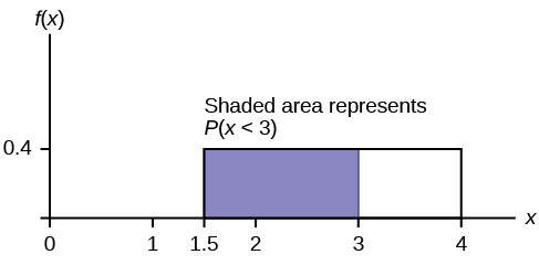
Probability of Repair Time Being Less Than Three Hours
Now, let’s find the probability that a repair requires less than three hours, i.e., (P(x < 3)). This is the area under the curve from 1.5 to 3.
(P(x < 3) = (text{base}) times (text{height}) = (3 – 1.5) times 0.4 = 1.5 times 0.4 = 0.6)
So, there’s a 60% probability that a furnace repair will be completed in less than three hours.
Uniform Distribution between 1.5 and four with shaded area between two and four representing the probability that the repair time x is greater than two
Determining the 30th Percentile of Repair Times
The 30th percentile is the value (k) such that 30% of the repair times are less than or equal to (k). Mathematically, we need to solve for (k) in (P(x leq k) = 0.30).
(P(x leq k) = (k – 1.5) times 0.4 = 0.30)
Solving for (k):
(k – 1.5 = frac{0.30}{0.4} = 0.75)
(k = 0.75 + 1.5 = 2.25)
Thus, the 30th percentile of furnace repair times is 2.25 hours. This implies that 30% of all repairs are completed in 2.25 hours or less.
Finding the Minimum Time for the Longest 25% of Repairs
We want to find the time duration that the longest 25% of repair times exceed. This is equivalent to finding the 75th percentile, or finding (k) such that (P(x > k) = 0.25).
(P(x > k) = (4 – k) times 0.4 = 0.25)
Solving for (k):
(4 – k = frac{0.25}{0.4} = 0.625)
(k = 4 – 0.625 = 3.375)
The longest 25% of furnace repairs take at least 3.375 hours. This also means that 3.375 hours is the 75th percentile of the repair times.
Mean and Standard Deviation of Uniform Distribution
Now, let’s focus on the mean and standard deviation of a uniform distribution. The mean ((mu)) of a uniform distribution (U(a, b)) is simply the average of the minimum and maximum values, given by:
(mu = frac{a+b}{2})
The standard deviation ((sigma)) measures the dispersion or spread of the distribution. For a uniform distribution (U(a, b)), the formula for the standard deviation is:
(sigma = sqrt{frac{(b-a)^{2}}{12}})
Calculating Mean and Standard Deviation for Furnace Repair Times
For our furnace repair time example, where (a = 1.5) and (b = 4):
Mean:
(mu = frac{1.5+4}{2} = frac{5.5}{2} = 2.75) hours
The average furnace repair time is 2.75 hours.
Standard Deviation:
(sigma = sqrt{frac{(4-1.5)^{2}}{12}} = sqrt{frac{(2.5)^{2}}{12}} = sqrt{frac{6.25}{12}} approx sqrt{0.5208} approx 0.7217) hours
The standard deviation of furnace repair times is approximately 0.7217 hours.
Interpretation of Standard Deviation in Uniform Distribution
The standard deviation of 0.7217 hours gives us a measure of the typical deviation of repair times from the mean of 2.75 hours. In a uniform distribution, unlike a normal distribution, the standard deviation doesn’t relate to specific percentages of data within one, two, or three standard deviations from the mean in the same way. However, it still provides a measure of the spread of the distribution. A larger standard deviation would imply a wider range between the minimum and maximum values in the uniform distribution, indicating greater variability in repair times.
In summary, understanding the standard deviation of a uniform distribution helps to quantify the variability within an equally likely range of outcomes. While the uniform distribution is simple, it’s a foundational concept in statistics, and grasping its properties, including the standard deviation, is crucial for more complex statistical analyses. For our furnace repair example, we’ve not only calculated the standard deviation but also seen how probabilities and percentiles are derived, offering a comprehensive view of working with uniform distributions.