
In statistics, the uniform distribution is a type of continuous probability distribution where every value within a specified interval has an equal chance of occurring. This means no value within the range is more likely than another. When visualized, this distribution takes the shape of a rectangle, which is why understanding the Uniform Distribution Graph is key to grasping this concept.
Unlike discrete distributions which can be shown with histograms, continuous distributions like the uniform distribution require a different visual approach. Since there are infinite possible values within a continuous interval, we represent probabilities using the area under a line or curve. For the uniform distribution, this line forms a rectangle over the defined interval.
Consider the uniform distribution graph illustrated below, which is set over the interval from 0 to 10. In this scenario, any number between 0 and 10 is equally likely to be observed. Values outside this range, less than 0 or greater than 10, have a probability of zero.
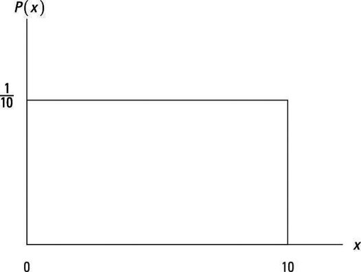 Uniform Distribution Graph Example: A rectangle illustrating a uniform distribution between 0 and 10, where all values in the interval are equally probable.
The range of values, from a lower limit (a) to an upper limit (b), defines the width of the rectangle in a uniform distribution graph. Mathematically, this width is calculated as b – a. In our example graph above, the width is 10 – 0 = 10. This width serves as the base of our rectangular representation.
The height of this rectangle is determined in such a way that the total area under the rectangle always equals 1. This is because in probability theory, the total probability of all possible outcomes must always be 1. To ensure this, the height of the rectangle in a uniform distribution graph is calculated as 1 divided by the base, or 1 / (b – a). In our example, the height is 1 / 10.
The area of any rectangle is found by multiplying its base by its height. For a uniform distribution graph, this means the area is ( b – a ) (1 / (b – a*)), which simplifies to 1. Crucially, any area under this rectangular graph represents a probability. For instance, the probability of a value falling within a specific sub-interval inside (0, 10) can be determined by calculating the area of the rectangle above that sub-interval.