
The uniform distribution is a cornerstone concept in probability and statistics, describing scenarios where all outcomes are equally likely over a certain range. Understanding the Uniform Distribution Equation is crucial for anyone working with probability, data analysis, or statistical modeling. This guide will delve into the intricacies of this distribution, providing clear explanations, practical examples, and insights into its applications.
What is Uniform Distribution?
At its heart, a uniform distribution, also known as a rectangular distribution, is a continuous probability distribution where every value within a defined interval has an equal chance of occurring. Imagine rolling a perfectly fair die – each face (1, 2, 3, 4, 5, or 6) has an equal probability of landing face up. While a die roll is a discrete example, the uniform distribution we’re focusing on here is continuous, meaning it deals with values that can fall anywhere within a range, not just distinct integers.
Think about waiting for a bus that arrives uniformly between 0 and 15 minutes past the hour. Any wait time within that 15-minute window is equally probable. This contrasts with other distributions where some outcomes are more likely than others, like a normal distribution where values cluster around the mean.
The Uniform Distribution Equation: Probability Density Function (PDF)
The core of the uniform distribution is its probability density function (PDF). This equation mathematically defines the distribution and allows us to calculate probabilities. For a uniform distribution, the PDF is remarkably simple:
f(x) = 1 / (b – a) for a ≤ x ≤ b
f(x) = 0 for x < a or x > b
Where:
- f(x) is the probability density function at a given value x.
- a is the minimum value of the distribution’s range.
- b is the maximum value of the distribution’s range.
This equation tells us that the height of the probability density function is constant within the interval [a, b] and zero outside of it. The value 1 / (b - a) ensures that the total area under the PDF curve over the interval [a, b] equals 1, which is a fundamental property of any probability density function (the total probability must be 1).
Let’s break down the components:
- (b – a): This represents the range or width of the uniform distribution.
- 1 / (b – a): This is the constant height of the PDF. A wider range (larger b – a) results in a lower height, and vice versa, maintaining the total area under the curve at 1.
Example: Baby Smiling Times
Consider the example from the original article about baby smiling times. It states that smiling times for an eight-week-old baby are uniformly distributed between 0 and 23 seconds, inclusive. Here, a = 0 and b = 23.
The probability density function for this scenario is:
f(x) = 1 / (23 – 0) = 1/23 for 0 ≤ x ≤ 23
f(x) = 0 for x < 0 or x > 23
This means that for any smiling time x between 0 and 23 seconds, the probability density is constant at 1/23.
Mean and Standard Deviation of a Uniform Distribution
Beyond the PDF, understanding the central tendency and spread of a uniform distribution is key. The mean (μ) and standard deviation (σ) provide this information.
Mean (μ)
The mean of a uniform distribution is simply the average of the minimum and maximum values:
μ = (a + b) / 2
This makes intuitive sense because the distribution is symmetric around the midpoint of the interval [a, b]. In our baby smiling example (a=0, b=23), the theoretical mean is:
μ = (0 + 23) / 2 = 11.5 seconds
This indicates that, on average, an eight-week-old baby smiles for 11.5 seconds, according to this uniform distribution model.
Standard Deviation (σ)
The standard deviation measures the spread or dispersion of the distribution. For a uniform distribution, the standard deviation is calculated as:
σ = √[(b – a)² / 12] = (b – a) / √12
In the baby smiling example (a=0, b=23), the theoretical standard deviation is:
σ = (23 – 0) / √12 ≈ 6.64 seconds
This value quantifies the typical deviation of smiling times from the mean of 11.5 seconds.
Calculating Probabilities with the Uniform Distribution Equation
One of the main uses of the uniform distribution equation is to calculate probabilities. For a continuous distribution, the probability of an event occurring within a specific interval is given by the area under the PDF curve over that interval. For a uniform distribution, this calculation simplifies to the area of a rectangle.
Probability P(c ≤ X ≤ d) where a ≤ c < d ≤ b:
P(c ≤ X ≤ d) = (base) (height) = (d – c) [1 / (b – a)] = (d – c) / (b – a)
Where:
- [c, d] is the interval for which we want to calculate the probability.
Example: Probability of Smiling Between 2 and 18 Seconds
Let’s revisit Example 5.3 from the original article. What is the probability that a randomly chosen eight-week-old baby smiles between 2 and 18 seconds? Here, c = 2 and d = 18.
P(2 ≤ X ≤ 18) = (18 – 2) / (23 – 0) = 16 / 23 ≈ 0.6957
This means there is approximately a 69.57% chance that a baby’s smiling time will fall between 2 and 18 seconds.
 Graph of Uniform Distribution for Baby Smiling Times with shaded area from x=2 to x=18, representing P(2 < x < 18)
Percentiles and the Uniform Distribution
Percentiles divide a dataset into 100 equal parts. The k-th percentile is the value below which k percent of the data falls. For a uniform distribution, percentiles are straightforward to calculate.
Finding the k-th Percentile (Pk):
Pk = a + k/100 * (b – a)
Where:
- k is the desired percentile (e.g., for the 90th percentile, k = 90).
Example: 90th Percentile of Smiling Time
Let’s find the 90th percentile for an eight-week-old baby’s smiling time (Example 5.3b). Here, k = 90, a = 0, and b = 23.
P90 = 0 + (90/100) (23 – 0) = 0.90 23 = 20.7 seconds
This indicates that 90% of baby smiling times are less than or equal to 20.7 seconds.
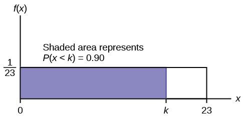 Graph of Uniform Distribution for Baby Smiling Times with shaded area to the left of k=20.7, representing 90th percentile
Conditional Probability and Uniform Distribution
Conditional probability deals with the probability of an event occurring given that another event has already occurred. With uniform distributions, conditional probabilities can be calculated by either adjusting the sample space or using the conditional probability formula.
Conditional Probability Formula:
P(A|B) = P(A and B) / P(B)
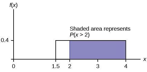
Example: Conditional Probability of Smiling Time
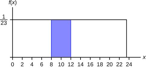
Consider Example 5.3c: Find the probability that a baby smiles more than 12 seconds knowing that the baby smiles more than eight seconds. Let A be the event (X > 12) and B be the event (X > 8).
Method 1: Adjusting the Sample Space
If we know the baby smiled more than 8 seconds, our new lower bound becomes 8, and the upper bound remains 23. The new uniform distribution is U(8, 23).
The probability density function becomes f(x) = 1 / (23 – 8) = 1/15 for 8 ≤ x ≤ 23.
P(X > 12 | X > 8) = P(X > 12 in U(8, 23)) = (23 – 12) / (23 – 8) = 11 / 15 ≈ 0.7333
Method 2: Using the Conditional Probability Formula
P(X > 12 | X > 8) = P(X > 12 and X > 8) / P(X > 8)
- P(X > 12 and X > 8) = P(X > 12) = (23 – 12) / 23 = 11 / 23
- P(X > 8) = (23 – 8) / 23 = 15 / 23
P(X > 12 | X > 8) = (11/23) / (15/23) = 11 / 15 ≈ 0.7333
Both methods yield the same result.
 Graph of Uniform Distribution for Baby Smiling Times with shaded area for conditional probability P(x > 12 | x > 8)
Real-World Applications of the Uniform Distribution Equation
While seemingly simple, the uniform distribution and its equation have applications in various fields:
- Simulation and Modeling: Used in Monte Carlo simulations when all values within a range are equally likely or when little is known about the underlying distribution.
- Random Number Generation: Computer algorithms often use uniform distributions as a base for generating other types of random numbers.
- Queuing Theory: Modeling wait times when service times or arrival times are uniformly distributed.
- Data Encryption: Sometimes utilized in cryptography for generating random keys or in noise generation.
- Quality Control: In scenarios where defects are uniformly distributed across a production line.
Conclusion
The uniform distribution equation is a fundamental tool for understanding and working with situations where outcomes are equally probable within a given range. Its simplicity makes it accessible, while its applications are surprisingly broad. By grasping the PDF, mean, standard deviation, and probability calculations associated with uniform distributions, you gain valuable insights for statistical analysis and problem-solving in diverse fields. Whether you are analyzing baby smiles, bus arrival times, or complex simulations, the uniform distribution equation provides a solid foundation for probabilistic reasoning.